
Visium Spatial Transcriptomics Tutorial
Full spatial analysis of a mouse brain coronal section — neighborhood enrichment, spatially variable genes, ligand-receptor interactions, and more.
What you'll learn
- Map transcriptomic clusters back onto the tissue section to recover anatomical structure (cortical layers, hippocampus, fiber tracts).
- Quantify which cluster pairs are spatially adjacent using neighborhood enrichment z-scores, and which genes are spatially structured using Moran's I.
- Detect spatial cell-cell signaling between neighbouring clusters using ligand-receptor analysis on the spatial graph.
Prerequisites
- • Oreumics installed (install guide).
- • Standard scRNA workflow familiarity — complete the PBMC tutorial first if Normalize → PCA → Leiden are unfamiliar.
- • Familiarity with AnnData and
obsm["spatial"]— defined inline in the glossary at the bottom of this page. - • Sample data:
sampledata/spatial/visium_mouse_brain.h5ad— pre-bundled, ~90 MB. - • Before the Ligand-Receptor step: install the OmniPath Intercell network once in the Resource Center and accept its licence. Oreumics never downloads a database in the middle of a run, so without it that one node stops with a “resource not ready” message while the rest of the workflow completes normally.
Overview
Spatial transcriptomics captures gene expression while preserving the physical location of each cell or spot in the tissue. This tutorial uses the 10x Visium Mouse Brain dataset — a coronal section of adult mouse brain with 684 tissue spots, the H&E image, scale factors and spatial coordinates pre-loaded. By the end you will have identified tissue regions, quantified cluster neighborhood enrichment, found spatially variable genes, and visualized ligand-receptor interactions.
Three templates covered
This page walks through the Spatial Full Analysis template in detail (15 analysis steps plus 7 Spatial Visualization nodes, in 5 phases). Two shorter templates — Spatial Neighborhood Analysis and Spatial Autocorrelation Scan — are covered at the end as quick-start variants.
Dataset
Sample file (pre-packaged in Oreumics)
sampledata/spatial/visium_mouse_brain.h5ad— 684 spots × 18,078 genes · ~90 MBWhat it contains
10x Visium coronal section of adult mouse brain (library V1_Adult_Mouse_Brain), converted from SpaceRanger output to H5AD. Spatial coordinates are in obsm['spatial'], the hires/lowres tissue images and scale factors are in uns['spatial'], and the file already carries a PCA, a UMAP and a 12-cluster obs['leiden'] from an earlier processing run. The full template recomputes these; the two short templates reuse them.
Spatial Full Analysis
Complete spatial pipeline: normalize → cluster → spatial graph → neighborhood enrichment → co-occurrence → spatially variable genes → Ripley statistics → ligand-receptor interactions → 7 visualization nodes. The pipeline is long; diagrams are split by phase.
Phase 1–2: Preprocessing + Dimensionality Reduction
Phase 3–4: Spatial Graph + Analyses (continued from Clustering)
Phase 5: Spatial Visualization fan-out from Ligand-Receptor
Phase 1 — Load Data
Load the mouse brain Visium file. It already contains spatial coordinates in obsm["spatial"] and the tissue image in uns["spatial"] — no additional coordinate loading is needed. (For your own SpaceRanger folder use the Load Visium (SpaceRanger) node instead — see "Tips for Your Own Visium Data".)
file_pathsampledata/spatial/visium_mouse_brain.h5adWhat you'll see
684 spots × 18,078 genes. obsm["spatial"] contains (x, y) pixel coordinates for every spot; uns["spatial"]["V1_Adult_Mouse_Brain"] holds the hires/lowres images and scalefactors.
Phase 2 — Standard Preprocessing
The preprocessing steps for Visium data are identical to scRNA-seq. Spatial coordinates are preserved throughout — they live in obsm and are unaffected by normalization or HVG selection. Note the template deliberately has no Scale node.
Scale every spot so that total counts equal target_sum. save_counts: true keeps the raw integer counts in adata.layers["counts"].
target_sum10000save_countstrueraw counts → layers["counts"]Apply log(x + 1) transformation. Compresses dynamic range and stabilizes variance so highly expressed genes do not dominate PCA.
basenullnatural log (default)Select the 2,000 most variable genes. Only HVGs are used for PCA, making the analysis both faster and more biologically meaningful. Spatial Autocorrelation later scans exactly this HVG set when its genes field is left empty.
n_top_genes2000flavorseuratWhat you'll see
2,000 genes flagged as highly_variable: True in adata.var.
Compute the top 50 principal components using only the HVGs.
n_comps50use_highly_variabletrueBuild a k-nearest-neighbor graph in PCA space. This graph is used by both UMAP (for layout) and Leiden (for clustering). n_pcs defaults to 15.
n_neighbors15use_repX_pcaCompute a 2D non-linear embedding for transcriptional similarity visualization. Note: UMAP uses transcriptional similarity — it will differ from the spatial tissue layout.
min_dist0.3Run Leiden community detection on the kNN graph. At resolution 0.5, the mouse brain section typically yields around 8–12 clusters corresponding to anatomical regions: cortical layers, hippocampus, fiber tracts, thalamus.
methodleidenresolution0.5key_addedleidenWhat you'll see
UMAP shows distinct clusters. Unlike PBMC data, clusters here correspond to tissue regions — each Visium spot averages several cells, so a cluster is an anatomical mixture rather than one cell type.
Tip
Adjust resolution to match expected tissue complexity. More anatomical regions = higher resolution.
Phase 3 — Spatial Neighborhood Graph
The Spatial Neighbors node builds a graph connecting physically adjacent spots on the tissue. This graph is the foundation for all downstream spatial analyses — neighborhood enrichment, co-occurrence, Ripley statistics, and ligand-receptor interactions all require it.
For Visium, use coord_type: grid — spots are arranged in a regular hexagonal grid (the node default "generic" is for single-cell platforms). n_rings: 1 means only immediate neighbors (6 for a hexagonal grid). delaunay: false uses the fixed grid topology rather than Delaunay triangulation. This spatial graph is stored in adata.obsp["spatial_connectivities"] and adata.obsp["spatial_distances"].
coord_typegriduse "generic" (default) for non-Visium datan_neighs6n_rings1only immediate neighborsdelaunayfalsespatial_keyspatialTip
For single-cell platforms (Xenium, MERSCOPE, CosMx) keep coord_type at "generic" and raise n_neighs to 10–20.
Compute which cluster pairs are significantly enriched in adjacent spots vs. random expectation. Uses a permutation test: for each permutation, cluster labels are randomly shuffled and the co-adjacency counts re-computed. The z-score compares the observed count to the permutation distribution.
cluster_keyleidenn_perms500node default 1000 for publication-quality p-valuesseed0What you'll see
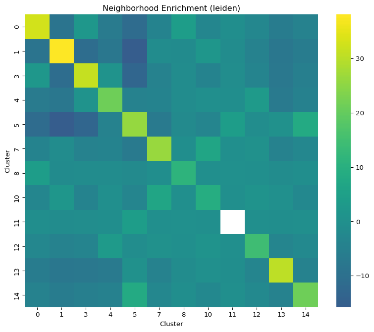
Results stored in adata.uns["nhood_enrichment"]. Strong positive z-scores = these clusters frequently appear in adjacent spots. Expect strong enrichment within anatomical regions (e.g., cortical layer clusters next to each other), and depletion across distant regions.
Calculate co-occurrence scores across increasing spatial distance ranges, showing which cluster pairs co-localize at different spatial scales. interval: 50 defines the step size (in coordinate units) for the distance bins.
cluster_keyleideninterval50What you'll see
Co-occurrence score curves per cluster pair stored in adata.uns["co_occurrence"]. Values > 1 = co-occurrence above chance. Curves reveal both local (short-range) and regional (long-range) spatial relationships.
Phase 4 — Spatial Statistics
Three statistical analyses that quantify spatial structure: Moran's I for spatially variable genes, Ripley's L for cluster spatial distribution, and squidpy's CellPhoneDB-style ligand-receptor permutation test between clusters. Each node adds its results to adata.uns so that all outputs are available when the visualization fan-out runs.
Compute Moran's I — a statistic between -1 and 1 where higher values indicate stronger spatial structure. This identifies spatially variable genes (SVGs) whose expression is not randomly distributed across the tissue. Leaving genes empty scans the highly variable genes; list gene names to test a custom set. Geary's C and sepal (grid-only diffusion time) are the other modes.
modemoranMoran's I spatial autocorrelationgenesn_jobs1What you'll see
Genes ranked by Moran's I stored in adata.uns['moranI']. In a coronal brain section the top hits are typically region-specific markers — myelin genes in fiber tracts, layer-specific cortical genes, hippocampal markers.
Ripley's L function tests whether each cluster is spatially clustered, dispersed, or random. Deviation above the simulated null = significant clustering. n_simulations: 50 controls the number of Monte Carlo simulations for the confidence envelope (node default 100).
cluster_keyleidenmodeLn_simulations50What you'll see
L-function curves per cluster stored in adata.uns. Clusters corresponding to compact anatomical structures deviate strongly upward; diffuse clusters track the null.
Runs squidpy ligrec — a CellPhoneDB-style ligand-receptor permutation test between clusters, using the OmniPath intercell ligand-receptor resource. That resource must already be installed in the Resource Center (licence accepted); the node will not fetch it mid-run. It scores on adata.raw when one exists (Scale sets it) and otherwise falls back to X with a warning — this template has no Scale node, so the log-normalized X is used. threshold: 0.01 retains interactions with permutation p-value < 0.01.
cluster_keyleidenn_perms500threshold0.01p-value threshold for significant pairsWhat you'll see
Significant ligand-receptor pairs between clusters stored in adata.uns["ligrec"]. Expect neuron–glia and neuron–vascular signalling pairs to dominate in brain tissue.
Tip
This node fans out to all 7 visualization nodes. It carries the full adata.uns with all upstream results, so every visualization has access to nhood_enrichment, co_occurrence, moranI, ripley, and ligrec results. Because this node is resource-gated, the 7 plots stay pending until OmniPath is installed — every node upstream still completes.
Phase 5 — Visualization (7 plots)
All seven Spatial Visualization nodes fan out from the Ligand-Receptor node, which carries the full adata.uns containing results from all four upstream spatial analyses. Each node produces an independent figure with its own Visualization Workspace — you can run all seven in parallel.
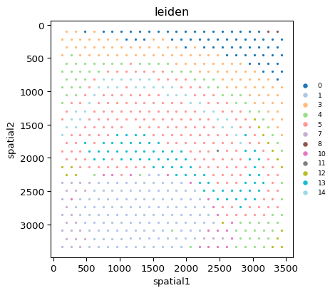
Shows the tissue section with each spot colored by its Leiden cluster over the H&E image. This is the most informative starting visualization — you can see how clusters map to anatomical brain regions. Use he_overlay for an image-first variant and alpha_img / bw to tune the tissue image.
plot_typespatial_scattercolor_byleidensize1.0cmaptab20What you'll see
A scatter of colored dots on the coronal brain section. Cortical layers appear as bands, the hippocampus as a curved arc, and fiber tracts as their own cluster between grey-matter regions.
Heatmap of neighborhood enrichment z-scores between all cluster pairs. Uses results from adata.uns["nhood_enrichment"] computed by the Nhood Enrichment node.
plot_typenhood_enrichmentcluster_keyleidentitleNeighborhood EnrichmentWhat you'll see
Symmetric heatmap of z-scores. Warm colors (positive z) = clusters frequently adjacent. Cool colors (negative z) = clusters rarely adjacent. Strong on-diagonal blocks confirm anatomical region coherence.
Line plots of co-occurrence scores across spatial distances. Uses adata.uns["co_occurrence"]. section_view and clusters control which groups are drawn.
plot_typeco_occurrencecluster_keyleidenWhat you'll see
Score curves per cluster pair. Values > 1 indicate co-occurrence above random chance at a given distance. Curves peaking at short distances = tight spatial co-localization; broad peaks = regional co-occurrence.
Summary of the Spatial Autocorrelation result — the genes with the highest Moran's I. Uses adata.uns['moranI'].
plot_typespatial_autocorrWhat you'll see
The top spatially variable genes ranked by Moran's I. Feed a top gene into a spatial_scatter node's color_by to see its pattern on the tissue.
Ripley's L curves for each cluster with the simulated null (show_null) and its interval band (show_interval). Deviation above the envelope = significant spatial clustering.
plot_typeripleycluster_keyleidenWhat you'll see
Line plots per cluster. Compact anatomical regions deviate strongly upward. Diffuse clusters track the null.
Dot plot of significant ligand-receptor pairs between clusters. Uses adata.uns["ligrec"]. source_groups / target_groups restrict the cluster pairs and pvalue_threshold hides weak interactions.
plot_typeligreccluster_keyleidenWhat you'll see
Dotplot matrix of significant interactions. Rows = cluster pairs, columns = ligand-receptor gene pairs. Large dark dots = strong, highly significant interactions.
A combined multi-panel summary of the spatial results for a quick look at the whole run.
plot_typespatial_overviewcluster_keyleidencolor_byleidenWhat you'll see
One figure summarising the tissue map alongside the spatial statistics. For a publication figure, drop the individual plots onto the Figure Canvas and arrange them there instead.
Shorter Templates
Two focused templates for when you only need a subset of the full analysis. Both rely on the obs["leiden"] column that the bundled file already carries.
Spatial Neighborhood Analysis
4-node pipeline focused on neighborhood enrichment. Assumes the H5AD already has cluster labels in obs[“leiden”] — true for the bundled file; for your own data run the clustering steps once and Save H5AD.
Pipeline
Load the Visium mouse brain file. This template assumes obs["leiden"] cluster labels are already present (12 clusters in the bundled file). If not, run the full Spatial Full Analysis pipeline first and save the H5AD after clustering.
file_pathsampledata/spatial/visium_mouse_brain.h5adBuild the spatial graph for the hexagonal Visium grid.
coord_typegridn_neighs6n_rings1delaunayfalsespatial_keyspatialPermutation test for cluster pair co-adjacency enrichment.
cluster_keyleidenn_perms500seed0Spatial Visualization node rendering the heatmap of neighborhood enrichment z-scores.
plot_typenhood_enrichmentcluster_keyleidenWhat you'll see
Heatmap of z-scores between all cluster pairs. Warm colors indicate clusters that frequently appear side-by-side in the tissue.
Spatial Autocorrelation Scan
4-node pipeline to find spatially variable genes (SVGs) using Moran's I. Run this when you want to quickly identify which genes have structured spatial expression patterns, without running the full clustering and neighborhood analysis.
Pipeline
Load the Visium mouse brain file.
file_pathsampledata/spatial/visium_mouse_brain.h5adBuild the spatial graph. Same parameters as the full pipeline.
coord_typegridn_neighs6spatial_keyspatialCompute Moran's I to rank genes by spatial structure strength. With genes left empty the node scans the highly variable genes stored in var (the bundled file already has an HVG flag).
modemorangenesn_jobs1What you'll see
adata.uns['moranI'] table ranked by Moran's I. Region-specific markers (myelin genes in fiber tracts, layer-specific cortical genes) rank at the top.
Spatial Visualization node. The template colors spots by leiden; set color_by to a specific gene name from the Moran's I table to see that SVG's pattern on the tissue section.
plot_typespatial_scattercolor_byleidenor replace with a gene namesize1.0cmapviridisWhat you'll see
Tissue scatter colored by leiden (or by a gene's expression if you set color_by to a gene name). Use the Moran's I table to pick the top SVG names.
Expected Results
- • Clusters at resolution 0.5: around 8–12 Leiden clusters corresponding to distinct mouse brain anatomical regions (the bundled pre-computed leiden has 12)
- • Neighborhood enrichment: Strong enrichment within anatomical regions — cortical layer clusters consistently appear adjacent to each other
- • Top SVGs: region-specific markers dominate the Moran's I ranking — confirms spatial structure is captured
- • Ligand-receptor: interactions between neighbouring clusters (neuron–glia, neuron–vascular) once OmniPath is installed
Tips for Your Own Visium Data
• Start from the SpaceRanger outs/ folder with the Load Visium (SpaceRanger) node (directory_path, counts: filtered, load_images: true). It reads the counts, the real coordinates, the true scalefactors and the H&E image in one go — attaching coordinates by hand forces placeholder scale values and silently disables the H&E overlay.
• For Visium HD use Load Visium HD and pick a bin size explicitly (8 µm recommended; 2 µm needs allow_2um and is guarded by max_bins).
• If you only have an expression matrix plus a coordinates CSV, use Add Coordinates (coords_file, x_col / y_col) to fill obsm["spatial"] — Spatial Neighbors, Ripley, Co-Occurrence and the Spatial Viewer all require obsm["spatial"], not obs columns.
• For single-cell platforms (Xenium, MERSCOPE, CosMx) keep coord_type in Spatial Neighbors at generic; grid is for Visium only.
• Adjust Clustering resolution to match expected tissue complexity — more regions = higher resolution. Spot Deconvolution (NNLS) against a labelled reference gives per-spot cell-type proportions when one label per spot is too coarse.
• Save H5AD after clustering to reuse the processed data in multiple spatial analysis runs without repeating preprocessing.
Going Further
- For single-cell-resolution spatial data (Xenium, MERSCOPE, CosMx), follow the Xenium tutorial — same pipeline but with
coord_type="generic". - Segment the section into contiguous tissue domains with Spatial Domains (BANKSY) (for Visium: spatial_weight 0.2, k_geom 18), and score where ligand–receptor pairs co-localize per spot with Spatial Ligand-Receptor.
- Use the Spatial Viewer to explore the section interactively (colour by gene or obs, lasso / box / polygon selection) and Spatial Grouping to turn drawn regions into an obs label for Subset Data.
- Extract per-spot H&E morphology descriptors with Spatial Image Features so texture and intensity can sit next to expression in the same table.
Glossary
- Visium
- A 10x Genomics spatial transcriptomics platform that captures gene expression at barcoded spots arranged in a hexagonal grid; each spot averages several cells depending on tissue density. Spot-based, not single-cell.
- obsm["spatial"]
- An n_spots × 2 array of (x, y) coordinates — full-resolution pixel coordinates for Visium, with the scale factors in uns["spatial"]. Read by all spatial-aware nodes.
- Spatial graph
- A neighbor graph built on physical proximity rather than transcriptional similarity. For Visium use coord_type="grid" with n_neighs=6 (hexagonal). Stored in obsp["spatial_connectivities"].
- Moran's I
- A statistic between -1 and +1 measuring spatial autocorrelation. +1 = strong spatial structure, 0 = random, —1 = checkerboard. Used to find spatially variable genes.
- Neighborhood enrichment
- A permutation test asking whether two clusters appear adjacent more often than chance. Z-scores summarize co-localization (positive) or avoidance (negative).