
Bulk RNA-seq Analysis
Differential expression and gene set enrichment analysis for bulk RNA-seq count data using the bundled airway excerpt — a dexamethasone-treated vs. control design in featureCounts format.
What you'll learn
- Load a featureCounts matrix + sample metadata, run sample-level QC, and normalize to log2(CPM+1).
- Test for differential expression between two conditions with PyDESeq2 and interpret a volcano plot.
- Translate the differential gene list into biological pathways using over-representation analysis (GSEA / ORA node, gseapy + Enrichr libraries).
Prerequisites
- • Oreumics installed (install guide).
- • Basic concept of RNA-seq counts — an integer per sample-by-gene table where each cell is a read count, conventionally produced by featureCounts, htseq-count, STAR, or salmon.
- • For Template 2: the GSEA / ORA node fetches Enrichr gene-set libraries online (listed as Enrichr Remote Analysis in the Resource Center — the one resource that is queried rather than installed). Only gene identifiers leave the machine; supply a local gene-set library if that is not acceptable.
- • Sample data:
sampledata/bulk/airway_featurecounts.txt+airway_metadata.csv— pre-bundled. Both templates on this page ship in the app as Bulk RNA-seq Differential Expression and Bulk RNA-seq with GSEA.
Dataset
Sample files (pre-packaged)
sampledata/bulk/airway_featurecounts.txt— Rsubread featureCounts output · 8 samples × 200 genes (Ensembl IDs)sampledata/bulk/airway_metadata.csv— sample metadata · columns: id, dex, celltype, geo_idsampledata/bulk/airway_rawcounts.csv— the same design as a plain genes × samples CSV for the Load Count Matrix node (enable transpose)What it is
A small teaching excerpt modelled on the Bioconductor airway experiment (human airway smooth muscle cells, dexamethasone vs. untreated; sample IDs SRR1039508–SRR1039521): four cell lines each treated or left untreated, giving 8 samples (4 control + 4 treated) in the dex column. The bundled counts cover only 200 genes with a differential signal built in, so it exercises the whole pipeline quickly — treat the biology as a demonstration, not as the published airway result.
Bulk RNA-seq Differential Expression
The core bulk RNA-seq pipeline: load featureCounts output, run sample QC, filter lowly-expressed genes, normalize, perform differential expression, and render a volcano plot (plus an MA plot) summarizing the results.
Pipeline
Load the airway featureCounts matrix alongside its sample metadata. The featureCounts format has two comment lines and several non-count columns (Chr, Start, End, Strand, Length) before the sample columns — the node skips these automatically and joins metadata rows to samples by sample_col. The same node also reads STAR ReadsPerGene.out.tab (strand_column picks the count column). Gene IDs become adata.var_names; sample IDs become adata.obs_names.
file_pathsampledata/bulk/airway_featurecounts.txtmeta_filesampledata/bulk/airway_metadata.csvsample_colidWhat you'll see
AnnData with 8 samples × 200 genes (Ensembl IDs). adata.obs contains the dex, celltype and geo_id columns from the metadata file. Raw integer counts are stored in adata.X.
Check per-sample quality metrics without removing samples. Evaluates library size (total read count), the number of detected genes, and IQR-based outliers. mode: label writes the metrics and an is_outlier flag to adata.obs rather than dropping samples, so you can inspect which samples — if any — failed before deciding to exclude them.
min_library_size100000require ≥100k total readsmin_detected_genes500require ≥500 detected genesmin_count_threshold1modelabelWhat you'll see
adata.obs gains library_size, n_genes_detected and is_outlier. With only 200 genes in the excerpt, the 500-gene floor is informational here — on a full matrix these defaults are sensible starting points.
Remove genes that are not expressed at a meaningful level in enough samples. CPM normalization is applied temporarily during filtering (from layers["counts"] when use_counts_layer is on) to make the threshold sample-size-independent. min_samples: 2 keeps genes detectable in at least 2 samples.
min_cpm1.0require ≥1 CPM in qualifying samplesmin_samples2must meet threshold in ≥2 samplesuse_counts_layertrueWhat you'll see
Genes below the expression floor are dropped; the node card reports the before/after gene count.
Normalize counts to CPM (counts-per-million), making cross-sample comparisons valid regardless of sequencing depth. log_transform: true applies log2(CPM + pseudocount); the pseudocount of 1.0 prevents log(0) for zero-count genes. Normalized values are stored in adata.X while raw counts are always preserved in adata.layers["counts"]. TMM, DESeq2 size factors and VST are the other methods.
methodcpmlog_transformtruepseudocount1.0What you'll see
adata.X now contains log2(CPM+1) values; layers["counts"] keeps the integers for PyDESeq2.
Tip
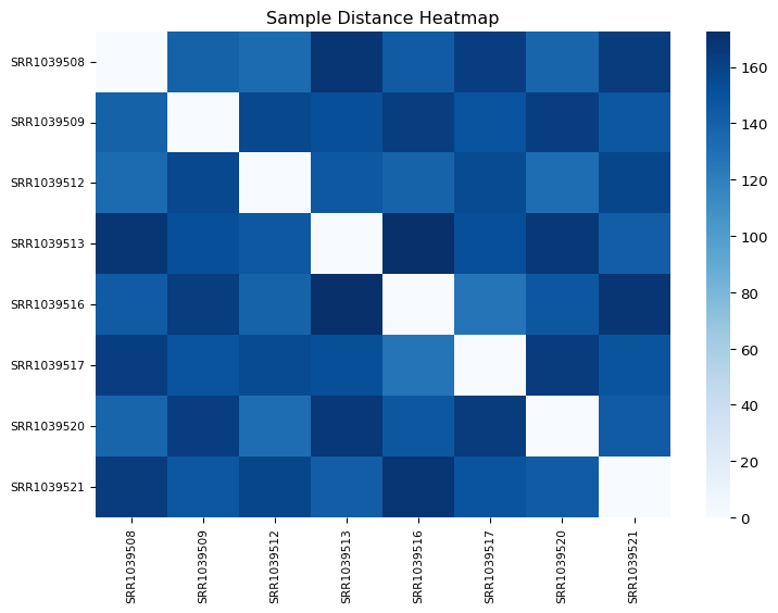
Add a Bulk Visualization node (plot_type: sample_dist, or library_size) after normalization to confirm samples cluster by treatment condition before running DE.
Test each gene for differential expression between the dexamethasone-treated and untreated conditions with PyDESeq2 (negative binomial; the node falls back to a t-test if PyDESeq2 cannot run). It reads the raw counts from layers["counts"]. reference_group and test_group are dropdowns populated from the values in condition_col — for the bundled metadata these are "control" and "treated". Positive log2 fold-change means higher in the test group. FDR is computed with the Benjamini–Hochberg procedure; genes passing alpha and |log2FC| ≥ lfc_threshold are flagged significant.
condition_coldexreference_groupcontroldenominatortest_grouptreatednumeratoralpha0.05lfc_threshold1.0≥2-fold minimum changemin_count10What you'll see
DE results table added to adata.uns["de_results"] with log2FC, p-value, padj and a significance flag per gene. The excerpt was built with a treatment signal, so a subset of the 200 genes comes out significant in both directions.
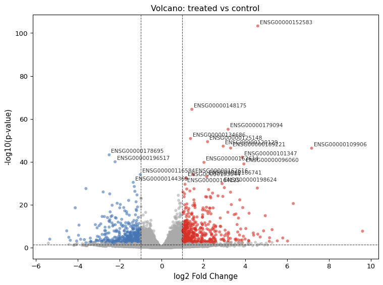
Plot a volcano chart summarizing the differential expression results. Each gene is placed at (log2 fold change, -log10 padj): significant upregulated genes appear in the upper-right, downregulated in the upper-left, and non-significant genes form a central gray cloud. n_label sets how many of the most significant genes get a name label; use_plotly switches to an interactive figure. The template adds a second node with plot_type: ma.
plot_typevolcanoalpha0.05lfc_threshold1.0n_label20genes to label (n_top_genes is for the heatmap)What you'll see
Volcano plot with two wings of significant genes flanking a gray cloud. Because var_names are Ensembl IDs, the labels are ENSG identifiers.
Bulk RNA-seq with GSEA
Extend the differential expression pipeline with gene set enrichment analysis (GSEA) or over-representation analysis (ORA) to identify enriched biological pathways in the DE gene list, then visualize the top DE genes as a heatmap and the sample-to-sample distances. This template uses a condensed pipeline (loading directly into DE) as a starting point.
Pipeline
Note: for a production analysis, insert the Bulk QC, Filter Low Expressed, and Bulk Normalize nodes between Load featureCounts and Differential Expression as shown in Template 1. The GSEA template uses a simplified pipeline for speed when exploring pathways on a pre-processed dataset.
Same as Template 1. Load the airway featureCounts matrix with the accompanying sample metadata.
file_pathsampledata/bulk/airway_featurecounts.txtmeta_filesampledata/bulk/airway_metadata.csvsample_colidRun DE with the same parameters as Template 1. The GSEA / ORA node reads the DE results table from adata.uns["de_results"], so this step must run first.
condition_coldexreference_groupcontroltest_grouptreatedalpha0.05lfc_threshold1.0min_count10Run over-representation analysis (ORA) on the significant DE gene list with gseapy. ORA tests whether the DE genes are more often annotated to a gene set than expected by chance. analysis_type: ora is faster than full GSEA and appropriate when the gene list is already filtered by significance; analysis_type: gsea instead ranks all genes (preranked GSEA, n_permutations). Enrichr libraries such as GO_Biological_Process_2023 are keyed by HGNC gene symbols — the bundled excerpt uses Ensembl IDs, so treat its enrichment output as a pipeline check rather than biology, and use symbol-named data (or a local gene-set library via gene_sets_custom) for real work.
analysis_typeoragene_setsGO_Biological_Process_2023organismHumanalpha0.05min_size10node default 15max_size500n_permutations1000used only for analysis_type: gseaWhat you'll see
Enrichment table stored in adata.uns["gsea_results"] (for both ORA and GSEA). On a real airway-style dataset with gene symbols, glucocorticoid-response and inflammatory-signalling terms are the kind of hits to expect among upregulated genes.
Tip
Switch gene_sets to KEGG_2021_Human for pathway-level results, or to MSigDB_Hallmark_2020 for curated gene set collections. For expression-based activity instead of a DEG-list test, see the PROGENy / Hallmark / CollecTRI activity nodes in Going Further.
Show the top DE genes across all 8 samples as a heatmap. n_top_genes picks the genes; alpha and lfc_threshold define which genes qualify as significant. The template pairs it with plot_type: sample_dist — a sample-to-sample distance matrix that should split the 4 control from the 4 treated samples.
plot_typeheatmapn_top_genes20alpha0.05lfc_threshold1.0What you'll see
A heatmap of the top DE genes with the 4 control and 4 treated samples forming two blocks; the sample-distance plot shows the same two-group structure.
Expected Results
- • Loaded matrix: 8 samples × 200 genes, obs columns dex / celltype / geo_id
- • Sample QC: library_size, n_genes_detected and is_outlier in obs; nothing removed in label mode
- • DE results: a subset of genes significant in each direction at FDR < 0.05 and |log2FC| > 1 — the exact counts are printed on the node card
- • Volcano / MA plots: two clear wings; heatmap and sample_dist split control from treated
- • ORA: a table in uns["gsea_results"]; meaningful terms need symbol-named genes
Tips & Troubleshooting
featureCounts file fails to load
Ensure the file has a header row with a "Geneid" column as the first column, followed by the annotation columns, then sample count columns. featureCounts adds leading "#" comment lines — the node handles them. Check the node error message for the specific column names it found.
No significant DE genes found
Confirm condition_col matches a column name in your metadata exactly (case-sensitive) and pick reference_group / test_group from the dropdown rather than typing them — for the bundled data the values are "control" and "treated". The Obs Inspector node (or the AI Copilot) shows value counts per column if you are unsure.
ORA returns no enriched terms
Enrichr libraries expect gene symbols. If adata.var_names are Ensembl IDs (as in the bundled excerpt), few or no genes will match a library; convert to symbols before loading, or point gene_sets_custom at a local library keyed the same way as your data.
Going Further
- Compare with single-cell-resolution differential expression in the PBMC DEG Analysis section.
- Score pathway activity rather than list over-representation with the PROGENy Activity (14 signalling pathways), Hallmark Activity (50 MSigDB programs) and CollecTRI TF Activity nodes — sample-level pseudobulk with sample_key, priors installed once from the Resource Center. See the Functional Activity node reference.
- Try the other loaders — the bundled
kallisto_abundance.tsvandsalmon_quant.sfboth load with Load Abundance (Kallisto/Salmon) (one sample per file — combine samples with Merge Data), andstar_ReadsPerGene.out.tabwith Load featureCounts (the STAR ReadsPerGene — Single-sample Load Demo template).
Glossary
- CPM (counts per million)
- A library-size normalization — each gene's count is divided by the sample's total reads × 1,000,000. Removes sequencing depth bias before comparing samples.
- PyDESeq2
- The Python implementation of DESeq2 that the Differential Expression node runs on the raw counts in layers["counts"], with condition_col as the design factor and reference_group as the baseline. A t-test is the fallback when it cannot run.
- log2 fold change (LFC)
- log2 of the ratio of expression between test and reference. LFC=1 means 2×, LFC=3 means 8×. Volcano-plot x-axis.
- FDR / adjusted p-value
- P-value corrected for multiple testing using Benjamini-Hochberg. The standard threshold is 0.05 — expect 5% of significant calls to be false positives.
- ORA (over-representation analysis)
- Statistical test that asks: are the genes in my DE list more often annotated to a pathway than expected by chance? Faster than full GSEA, which instead walks the full ranked gene list.