
ATAC-seq Tutorial
Chromatin accessibility analysis with differential accessibility and motif discovery on the bundled Cell Ranger ATAC MEX demo.
What you'll learn
- Load a Cell Ranger ATAC peak-barcode matrix and judge library quality from fragment counts and FRiP.
- Reduce dimensions with LSI (TF-IDF + SVD) instead of PCA, cluster on the LSI-derived neighbor graph, and detect peaks with significantly altered chromatin accessibility between clusters.
- Discover transcription factor (TF) motifs enriched in those differentially accessible peaks using JASPAR (2022 by default, releases up to 2026 selectable).
Prerequisites
- • Oreumics installed (install guide).
- • Conceptual familiarity with scRNA clustering — ATAC-seq reuses the same Neighbors → Leiden flow with one critical change (use_rep=X_lsi instead of X_pca).
- • Peaks, FRiP, and LSI are defined in the glossary at the bottom of this page.
- • Sample data:
sampledata/atac/filtered_peak_bc_matrix/— pre-bundled, Cell Ranger ATAC MEX format. Both templates on this page ship in the app as ATAC Differential Accessibility and ATAC Motif Discovery. - • Motif Analysis uses the JASPAR releases bundled with the installer (pyJASPAR; tracked as a bundled entry in the Resource Center) — nothing to download. Scanning your own peak sequences additionally needs a genome FASTA, supplied through the node's genome_fasta parameter.
Dataset
Sample files (pre-packaged)
sampledata/atac/filtered_peak_bc_matrix/— Cell Ranger ATAC MEX layout: matrix.mtx.gz, peaks.bed, barcodes.tsv.gz · 200 barcodes × 2,000 peakssampledata/atac/pbmc500_atac.h5ad— 10x PBMC 500 scATAC peak matrix, 623 cells × 47,843 peaks (Load H5AD or Load Peak Matrix)sampledata/atac/fragments_demo.tsv— fragments-format demo subset for Load Fragments (not bgzipped)What it is
The MEX directory used by both templates is a small demo in the exact Cell Ranger ATAC filtered_peak_bc_matrix layout — the same three-file structure as 10x scRNA-seq output, but the features are genomic peak regions (chr:start-end) instead of gene names. It is sized to run the whole pipeline quickly; for a realistic dataset swap in the bundled PBMC 500 H5AD or your own Cell Ranger ATAC output.
Key Concept — LSI vs PCA
ATAC-seq data is highly sparse (most peaks are 0 for any given cell). PCA performs poorly on this type of data. Instead, Oreumics uses LSI (Latent Semantic Indexing): it first applies TF-IDF normalization to down-weight ubiquitous peaks, then performs a randomized SVD. The first LSI component typically correlates with sequencing depth rather than biology — always keep drop_first: true (the default) to remove it.
ATAC Differential Accessibility
Load the ATAC MEX data, run QC and peak selection, reduce dimensions with LSI, cluster cells by chromatin state, then identify peaks that are significantly more or less accessible between two clusters using a statistical test.
Pipeline (scroll →)
Load the peak-barcode matrix in MEX (Market Exchange) format — the same format as 10x Genomics scRNA-seq output but with genomic peaks (peaks.bed) as features instead of genes.
directory_pathsampledata/atac/filtered_peak_bc_matrixWhat you'll see
200 cells × 2,000 peaks loaded into AnnData. The var index contains peak coordinates (e.g., chr1:827166-827716).
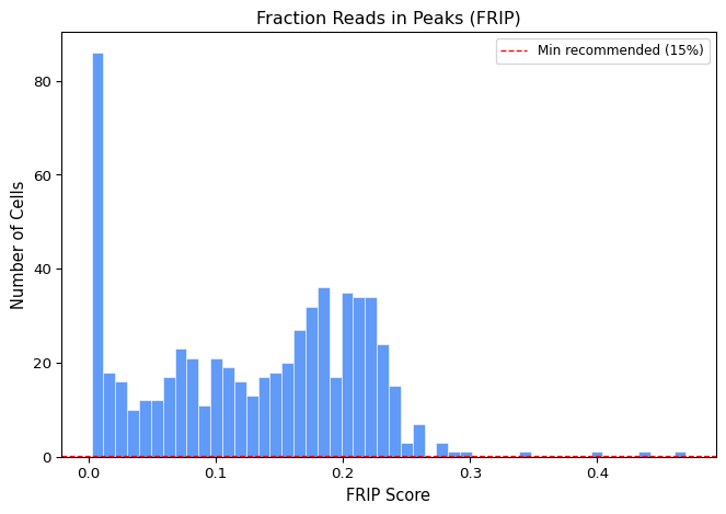
Compute per-cell QC metrics and label low-quality cells. FRiP (Fraction of Reads in Peaks) is the primary ATAC-seq QC metric — cells with FRiP below 0.15 have poor signal-to-noise. Using mode: label marks low-quality cells without removing them, so you can inspect the distribution first.
min_total_fragments1000max_total_fragments100000filters potential doubletsmin_frip0.15ENCODE recommends ≥0.20 for bulk; ≥0.15 for scmodelabelWhat you'll see
obs gains total_fragments, n_peaks_detected, frip_approx and a pass/fail label. The number of cells passing is reported on the node card (the demo matrix is small, so do not read biology into it).
Select the most accessible peaks across all cells. method: top_accessible keeps the keep_top_n most accessible regions and is the fast default; method: macs3 calls peaks with MACS3 (genome_size and q_value apply there, with keep_top_n as a cap on the output). Reducing to 500 peaks keeps computation fast on the demo dataset; for production analyses increase keep_top_n.
methodtop_accessiblekeep_top_n500genome_sizehsMACS3 only; use mm for mouseq_value0.01MACS3 onlyWhat you'll see
adata.var filtered to 500 peaks. adata.shape is now (n cells) × 500 peaks.
Compute the LSI embedding using TF-IDF normalization followed by randomized SVD. scale_factor and log_transform replicate the standard normalization built into ATAC LSI workflows. drop_first: true is critical — LSI component 1 almost always captures sequencing depth differences, not biology.
n_components30node default 50scale_factor10000log_transformtruedrop_firsttrueremoves depth-correlated componentWhat you'll see
adata.obsm["X_lsi"] created. The remaining components capture biological variation.
Tip
If clustering looks poor, try increasing n_components to 50 and use the first 20 in Neighbors (n_pcs).
Build a k-nearest-neighbor graph in LSI space. This is the most important difference from an scRNA-seq workflow: you must specify use_rep: X_lsi to use the LSI embedding instead of the default X_pca. The neighborhood graph drives both UMAP layout and Leiden clustering.
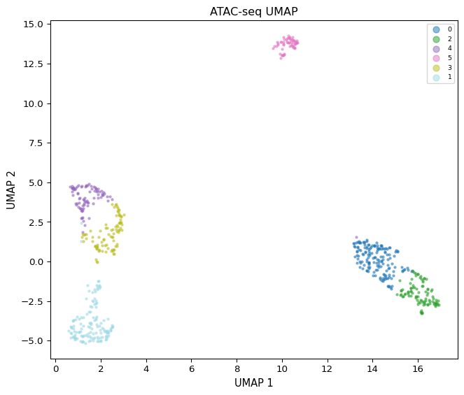
n_neighbors15use_repX_lsicritical — do not leave as X_pcaCompute a 2D embedding from the LSI-based neighbor graph so clusters can be viewed with ATAC Visualization (plot_type: umap_atac).
min_dist0.3Run Leiden community detection on the kNN graph. Resolution 0.5 produces a moderate number of clusters for the demo dataset. Increase to 0.8–1.2 for larger datasets or finer cluster resolution.
methodleidenresolution0.5key_addedleidenWhat you'll see
A few clusters labeled 0, 1, 2… in obs["leiden"].
Run a statistical test (t-test + FDR) comparing peak accessibility between two clusters. Peaks passing alpha and log2fc_threshold are classified as significantly differentially accessible. min_pct: 0.05 filters out peaks open in fewer than 5% of cells in either group. Cluster labels are strings — pick reference_group and test_group from the dropdown values that Leiden assigned.
groupbyleidenreference_group0test_group1alpha0.05log2fc_threshold1.0min_pct0.05What you'll see
uns["chrom_access_results"] stores a table with log2FC, p-value, FDR and a significance flag per peak; the count of significant peaks is shown on the node card.
plot_type: differential renders a volcano plot with log2 fold-change on the x-axis and -log10(p-value) on the y-axis; the most significant peaks are annotated with their genomic coordinates. The template adds a second node with plot_type: umap_atac and color_by: leiden. Other plot types: frip_bar, fragment_size, tss_enrichment, peak_accessibility.
plot_typedifferentialn_top_peaks100peaks highlighted / shown in heatmapWhat you'll see
Volcano plot separating peaks more accessible in the test cluster from peaks more accessible in the reference cluster. Annotated peaks show genomic loci (e.g., chr1:1234567-1235067) which can be looked up in genome browsers.
ATAC Motif Discovery
The same chain as Template 1 (without the UMAP node) plus motif enrichment on the differentially accessible peaks. Motif Analysis scans your DA peaks against a JASPAR release to identify which transcription factor (TF) binding motifs are enriched at open chromatin loci — suggesting those TFs may be active in that cell population.
Additional nodes (after Chrom Accessibility)
Key Concept — JASPAR
JASPAR is a curated database of position-frequency matrices (PFMs) for transcription factor binding sites, published in dated releases. Motif Analysis scans your differentially accessible peaks against the motifs of the chosen release and returns enrichment scores. High enrichment means that TF's binding motif appears more often in your open peaks than expected by chance — suggesting that TF may be active in those cells.
Scan the top differentially accessible peaks against JASPAR (via pyJASPAR) to find enriched TF binding motifs. database defaults to JASPAR2022 so existing analyses keep reproducing exactly; releases from JASPAR2020 through JASPAR2026 are bundled and selectable. genome_fasta is optional: leave it blank and the node uses peak sequences pre-cached in adata.uns when present, otherwise it falls back to ranking by peak statistics only. For your own data, provide a FASTA for your assembly (hg38.fa, mm10.fa, …) to get real sequence scanning. alpha: 0.05 filters the reported motifs.
databaseJASPAR2022JASPAR2020 … JASPAR2026 availablegenome_fastan_top_peaks500alpha0.05What you'll see
uns["motif_results"] contains a table of enriched TF motifs with enrichment score and adjusted p-value. On real PBMC chromatin, immune-lineage TF families are the kind of hit to expect; the synthetic demo only proves the plumbing.
Tip
For real datasets, always provide a genome_fasta path matching your reference assembly to get accurate motif scanning results.
Render a heatmap of chromatin accessibility across the top peaks for each cluster. Rows are peaks, columns are clusters. Color intensity reflects accessibility level (higher = more open). This complements the volcano plot by showing the accessibility landscape across all clusters simultaneously.
plot_typepeak_accessibilityn_top_peaks100What you'll see
Heatmap with cluster-specific open chromatin regions appearing as bands of high accessibility in one column but low in others.
Expected Results
- • Loaded matrix: 200 cells × 2,000 peaks from the MEX demo
- • After ATAC QC: total_fragments, n_peaks_detected, frip_approx and a pass label in obs; nothing removed in label mode
- • LSI: 30 components computed; drop_first removes the depth-correlated component
- • Leiden at resolution 0.5: a few clusters on the demo; more on real data
- • Differential accessibility: a table in uns["chrom_access_results"] with significant peaks between cluster 0 and cluster 1 at α = 0.05 and |log2FC| > 1
- • Volcano plot: distinct point clouds; top annotated peaks give loci to look up
- • Motif analysis (Template 2): a ranked motif table in uns["motif_results"]
- • Peak accessibility heatmap: cluster-specific banding of open chromatin regions
ATAC-seq Tips
Always set use_rep: X_lsi in Neighbors
The Neighbors node defaults to X_pca. For ATAC-seq you must set use_rep to X_lsi. Forgetting this is the most common mistake — without a PCA upstream the node cannot build the graph you intended.
Choosing reference_group and test_group
Cluster labels are strings. If Leiden assigns labels 0, 1, 2… set reference_group: 0 and test_group: 1 from the dropdown. Positive log2FC means the peak is more accessible in the test group; negative means more accessible in the reference group.
FRiP threshold guidance
The ENCODE project recommends FRiP ≥ 0.20 for bulk ATAC. For single-cell ATAC the threshold is typically relaxed to 0.15 due to lower per-cell coverage. Datasets with many cells below 0.15 may indicate library quality issues.
Going Further
- Start from other inputs: Load Fragments builds a peak × cell matrix from a 10x fragments.tsv.gz (calling peaks or binning when no BED is given), and Load Peak Matrix reads a pre-computed CSV / H5AD such as the bundled pbmc500_atac.h5ad.
- Run the Pathway Enrichment tutorial on the genes nearest to your differentially accessible peaks to get pathway-level interpretation.
- Use the AI Copilot (right-side chat panel) to interpret specific peak coordinates — e.g., "what gene is closest to chr1:1234567-1235067?" — and to read the differential and motif tables back to you.
Glossary
- Peak
- A region of the genome where Tn5 transposase inserted more often than chance — an open, accessible chromatin region. Peaks are called by Cell Ranger ATAC or MACS3 (the Peak Calling node) and stored in the var index of the AnnData (e.g., chr1:827166-827716).
- FRiP (Fraction of Reads in Peaks)
- A library quality metric: the fraction of a cell's sequencing reads that fall inside called peaks. ENCODE recommends >=0.20 for bulk; >=0.15 is the sc-ATAC threshold. Stored as frip_approx by ATAC QC.
- LSI (Latent Semantic Indexing)
- TF-IDF normalization followed by SVD — the ATAC-seq replacement for PCA. The first LSI component almost always captures library depth, so keep drop_first=true.
- TSS enrichment
- Ratio of fragment density at transcription start sites vs. flanking regions. A second core ATAC quality metric; ATAC Visualization has a tss_enrichment plot type.
- JASPAR
- A curated database of transcription factor binding motifs (PFMs), released in dated versions. Motif Analysis scans your differentially accessible peaks for enrichment of these motifs; JASPAR2022 is the default, JASPAR2020–2026 are bundled.