
PBMC scRNA-seq Tutorial
Complete single-cell RNA-seq walkthrough — QC, normalization, clustering, and marker discovery using the 10x Genomics PBMC 3k dataset.
What you'll learn
- Inspect a raw scRNA-seq dataset in the QC Workspace, decide on QC thresholds from violin plots, and remove low-quality / dying cells.
- Run the standard normalize → log1p → HVG → scale → PCA → neighbors → UMAP → Leiden pipeline and interpret the cluster layout.
- Rank each Leiden cluster's marker genes with DEG Analysis and annotate cell types (T cells, B cells, NK cells, monocytes, DCs, platelets).
Prerequisites
- • Oreumics installed and running (install guide).
- • Quick Start completed — you should know how to drag a node, connect edges, and click Run.
- • Familiarity with AnnData — the cells × genes container that Oreumics nodes pass between each other (defined inline in the glossary at the bottom of this page).
- • Sample data:
sampledata/scrna/pbmc3k_raw.h5ad— pre-bundled, no download needed.
Dataset
Sample file (pre-packaged)
sampledata/scrna/pbmc3k_raw.h5ad— 2,700 cells × 32,738 genes · integer counts · already included in OreumicsWhat it is
Peripheral blood mononuclear cells (PBMCs) from a healthy human donor, sequenced on a 10x Chromium v2 chip. Contains T cells, B cells, NK cells, monocytes, dendritic cells, and platelets. Standard reference dataset for learning scRNA-seq analysis. Despite the _raw in the file name it is the Cell Ranger filteredmatrix (empty droplets already removed) converted to H5AD; obs is empty until the Quality Control node adds its metrics.
scRNA QC Overview
A 2-node pipeline that computes per-cell quality metrics and renders the built-in violin plot without removing anything. Run this before any filtering to inspect the raw distributions and decide on QC thresholds. The old separate QC Metrics and QC Visualization nodes are merged into the single Quality Control node.
Pipeline
Load the PBMC 3k counts. Do NOT apply any filtering yet — doublet detection and QC inspection should always run on unfiltered data.
file_pathsampledata/scrna/pbmc3k_raw.h5adWhat you'll see
2,700 cells × 32,738 genes loaded. obs is empty (the barcode is the index); the next node fills it.
Compute per-cell quality metrics and draw the built-in violin plot without removing any cells. mode: label only marks cells; the template additionally switches every filter toggle off so nothing is flagged yet. Adds n_genes_by_counts, total_counts, pct_counts_mt, pct_counts_ribo and pct_counts_hb to obs.
modelabelmito_prefixMT-human mitochondrial genes ("mt-" for mouse)ribo_prefixRPS,RPLribosomal protein geneshb_prefixHBhemoglobin genesfilter_min_genesfalsefilter_max_pct_mitofalsefilter_min_cellsfalseshow_plottrueplot_typeviolinmetrics["n_genes_by_counts", "total_counts", "pct_counts_mt"]defaultWhat you'll see
Three violin panels on the node card. n_genes_by_counts: most cells have 500–2,000 genes; a few near 0. pct_counts_mt: most cells <10%; dying cells cluster near 20–50%. Use these to set min_genes and max_pct_mito in the next template.
Tip
Open the QC Workspace from the node (toolbar button). It shows MAD-based "rec:" threshold recommendations, a Raw Data Mode for unfiltered Cell Ranger output, and re-draws the thresholds live — no re-run needed until you press Apply.
scRNA Standard Clustering
The full preprocessing → dimensionality reduction → clustering pipeline (12 nodes). Starting from raw counts, produces a UMAP colored by Leiden clusters — the foundation of every scRNA-seq analysis.
Pipeline (scroll →)
Load the PBMC 3k counts file.
file_pathsampledata/scrna/pbmc3k_raw.h5adFilter out low-quality cells (empty droplets, dying cells) and lowly-detected genes. mode: filter removes cells permanently; use mode: label to only mark them first. Each threshold has its own enable toggle.
modefilterfilter_min_genestruemin_genes200remove empty dropletsfilter_max_pct_mitotruemax_pct_mito20remove dying cellsmito_prefixMT-filter_min_cellstruemin_cells3remove genes seen in <3 cellsWhat you'll see
~2,638 cells and ~13,714 genes remain after filtering.
Scale every cell so that the total count equals target_sum, removing library-size differences. save_counts: true keeps the raw integer counts in adata.layers["counts"] for anything that needs them later (e.g. seurat_v3 HVG selection or a DESeq2-style test).
target_sum10000save_countstrueraw counts → layers["counts"]Apply log(x + 1) transformation. Compresses the dynamic range and stabilizes variance, so highly expressed genes do not dominate PCA. save_normalized keeps a copy in layers["normalized"].
basenullnatural log (default)save_normalizedtrueSelect the 2,000 most variable genes. Only HVGs are used for PCA, making the analysis both faster and more biologically meaningful. flavor "seurat" works on the log-normalized matrix; "seurat_v3" expects raw counts (point layer at "counts").
n_top_genes2000flavorseuratWhat you'll see
2,000 genes flagged as highly_variable: True in adata.var.
Standardize each gene to zero mean and unit variance, capped at max_value: 10 so outlier cells do not distort PCA. With hvg_only: true (the default since v0.15.0) X is reduced to the ~2,000 HVGs, which is all PCA needs; the full log-normalized gene set is saved automatically to adata.raw, which DEG Analysis and the plots read.
max_value10zero_centertruehvg_onlytruedefault; full genes kept in adata.rawCompute the top 50 principal components using only the HVGs. Captures the major axes of variation in the data.
n_comps50use_highly_variabletrueTip
Add a PCA Visualization node (plot_type: variance_ratio) after PCA to find the "elbow" — use that number of PCs for n_pcs in Neighbors.
Build a k-nearest-neighbor graph in PCA space. This graph is used by both UMAP (for layout) and Leiden (for clustering). The node default is n_pcs 15; 0 means use every PC.
n_neighbors15use_repX_pcan_pcs30default 15 — or use your elbow estimateCompute a 2D non-linear embedding for visualization. Lower min_dist packs clusters tighter; higher values spread them out (node default 0.1).
min_dist0.3spread1.0Run Leiden community detection on the kNN graph. Increase resolution for more clusters; decrease for fewer (node default 1.0). Louvain and K-Means (method: kmeans + n_clusters, partitions the PCA embedding) are also available.
methodleidenresolution0.8key_addedleidenWhat you'll see
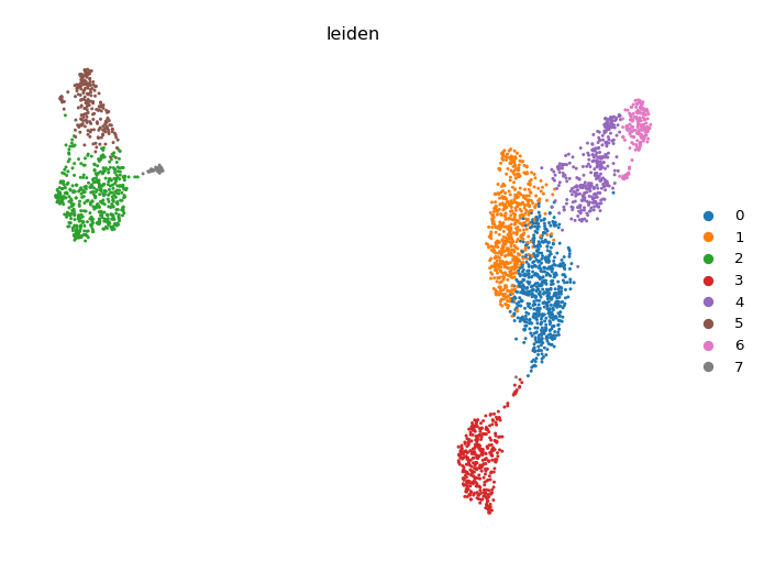
7–9 clusters (labeled 0–7 or 0–8). In the UMAP colored by leiden, expect distinct islands: 2–3 T cell clusters, 1 B cell cluster, 1 NK cluster, 1–2 monocyte clusters, and small DC/platelet clusters.
Plot the composition (cell count) of each Leiden cluster as a bar chart. Note that "umap" is not a plot_type here — use plot_type: embedding + embedding: umap for a cluster overlay, or the Embedding Plot node below.
plot_typecompositioncluster_keyleidenWhat you'll see
Bar chart of cluster sizes. Monocyte clusters (LYZ+) are typically the largest non-T-cell population.
UMAP scatter colored by an obs column or a gene. color_by accepts comma-separated columns; gene_symbols overlays expression (layer "auto" reads adata.raw so you see log-normalized values, not z-scores).
plot_typeumapcolor_byleidenWhat you'll see
The canonical UMAP colored by Leiden cluster. Open the Visualization Workspace on this node to rename groups, change per-group colours, or move the legend without re-running the analysis.
scRNA Marker Discovery
Extends the Standard Clustering pipeline with the nodes that rank and visualize the top marker genes per cluster. Run after completing Template 2 or use the scRNA Marker Discovery template, which skips Quality Control for brevity, clusters at resolution 1.0, and ends in a dotplot plus a heatmap.
Additional nodes (after Clustering)
Differential expression for each cluster vs. all other cells using the Wilcoxon rank-sum test (formerly named "Find Markers"; the node id is still findMarkers). Leave n_genes empty to rank ALL genes — the plots and the Top DEG Gene List node pick their own top-N later. use_raw reads adata.raw (set by Scale), and pts adds the fraction of cells expressing each gene in the group vs. the rest. Results are stored in adata.uns["rank_genes_groups"].
groupbyleidenmethodwilcoxonn_genesnullempty = all genes (recommended)referencerestuse_rawtrueptstruepct_nz_group / pct_nz_referenceWhat you'll see
Ranked genes per cluster with scores, log fold changes and adjusted p-values. Key markers expected: CD3D/CD3E (T cells), MS4A1/CD79A (B cells), NKG7/GNLY (NK), LYZ/CST3 (monocytes), PPBP (platelets).
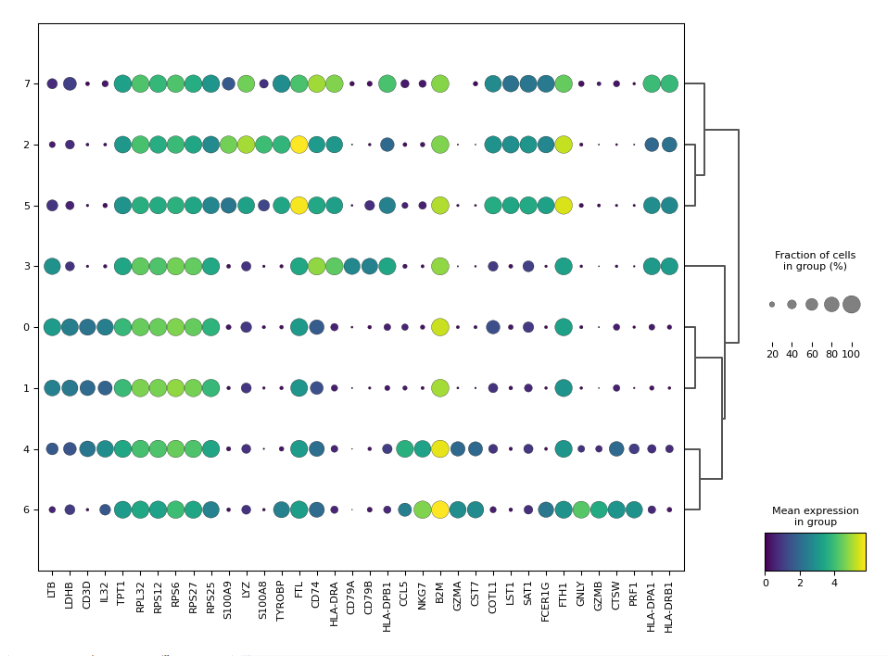
Visualize the top N marker genes per cluster. rank_genes_groups_dotplot is the most informative: dot size = fraction of cells expressing the gene, color = mean expression.
plot_typerank_genes_groups_dotplotn_genes5top 5 per clustergroupbyleidenWhat you'll see
Dotplot matrix (clusters × top genes). Each row is a cluster; columns are genes. Large dots in a row = that gene is a strong marker for that cluster. CD3D large in T cell rows, LYZ large in monocyte rows — use these patterns to annotate cell types.
Tip
The template adds a second Marker Visualization with plot_type: rank_genes_groups_heatmap for a per-cell view. With many genes, switch on figsize_auto so the figure grows with the grid instead of squeezing labels.
Expected Results
- • After QC: ~2,638 cells remain (from 2,700); ~13,714 genes
- • Clusters at resolution 0.8: 7–9 Leiden clusters
- • Cell types: CD4 T cells (CD3D+, IL7R+), CD8 T cells (CD3D+, CD8A+), B cells (MS4A1+, CD79A+), NK cells (NKG7+, GNLY+), CD14 Monocytes (LYZ+, CST3+), FCGR3A Monocytes, Dendritic cells (FCER1A+)
- • UMAP: Clear separation between lymphoid (T/B/NK) and myeloid (monocyte/DC) lineages; T cell subclusters visible at higher resolution
Going Further
- Turn cluster numbers into cell-type names with Edit Clusters (rename/merge rules), or let Auto Annotation (LLM, per cluster) or CellTypist Annotation (pretrained model, per cell; model installed once via the Resource Center) do it, then check agreement with Annotation Concordance.
- Run Pathway Enrichment on the marker genes to discover the biological processes active in each cluster.
- Add a second sample and integrate batches with the Harmony tutorial.
- Reconstruct cell differentiation paths through the same data using the PAGA + DPT trajectory tutorial.
Glossary
- AnnData
- An annotated data matrix — cells (rows) × genes (columns) with side panels for cell metadata (obs), gene metadata (var), embeddings (obsm), and unstructured results (uns). The standard container that flows between Oreumics nodes.
- HVG (highly variable genes)
- Genes whose expression varies the most across cells — the genes that carry biological signal. Selected after Log1p; only HVGs are used for PCA, and Scale keeps only them in X while preserving every gene in adata.raw.
- Leiden clustering
- A community detection algorithm that partitions the kNN graph into densely connected subgroups.
resolutioncontrols granularity: higher = more, smaller clusters. - UMAP
- A 2D non-linear embedding for visualization. Distances on the UMAP roughly reflect transcriptional similarity but are not metric — trust clusters, not exact distances.
- DEG (differentially expressed gene)
- A gene that is significantly more (or less) expressed in one cluster vs. the rest, as ranked by the DEG Analysis node. Used to annotate cell types.