
Visium, Visium HD, Xenium, MERSCOPE and CosMx — loaded natively, analysed in one canvas.
5 native platform loaders plus transcripts and CSV coordinates. An interactive Plotly viewer with lasso, box and polygon selection turns regions into obs labels; BANKSY segments tissue into domains; cellular neighborhoods type microenvironments; squidpy supplies neighborhood enrichment, co-occurrence, Moran’s I / Geary’s C / sepal and Ripley statistics — drawn with 16 spatial plot types.
In the Spatial view
- Nodes in this view
- 50
- Loaders
- 10
- Templates
- 4
- Plot types
- 16
10 pipeline stages
Visium (SpaceRanger) · Visium HD · Xenium · MERSCOPE …
1 need a Resource Center install
across the visualization nodes in this view
Counted from the app’s v0.25 Node Library view, not typed by hand.
SpaceRanger outs/
spots × genes + H&E
min_genes 200
QC_label set
leiden · resolution 1.0
clusters
coord_type grid · 6 hex
graph built
perms 1000
z-scores
BANKSY · λ 0.2 · k 18
spatial_domain
spatial_scatter
figure ready
A Spatial pipeline on the Oreumics canvas — drag, connect, run. Illustration; parameters are examples.
What it produces
Result capture
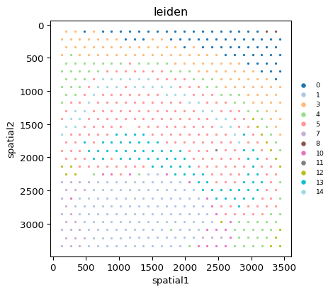
Spatial Visualization, spatial_scatter plot type — Leiden clusters drawn in tissue coordinates on the bundled Visium mouse-brain section.
What you can drag in.
dirA whole SpaceRanger folder: counts, real spot coordinates, the true scalefactors and the H&E image, so overlays and micron scale bars work.
dirOne square-bin resolution (2, 8 or 16 µm; 8 recommended, 2 µm needs an explicit opt-in) with a bin-count guard applied before anything is read.
dircell_feature_matrix.h5 (or the MEX directory) aligned with cells.parquet / csv micron centroids; controls dropped by default.
.csvcell_by_gene and cell_metadata CSV (.gz OK) with micron coordinates and an optional coordinate transformation; Blank probes kept in their own slot.
.csvFlat cell-by-gene and metadata exports; FOV + cell ID pairing with slide-wide global coordinates as the canonical system.
.parquetSingle-molecule transcript tables from Xenium / MERFISH / seqFISH (parquet preferred for Xenium) for density and dot overlays.
.csvStand-alone X / Y for any platform; column names such as x_centroid or pxl_col_in_fullres are auto-detected.
.h5adAn .h5ad that already carries obsm["spatial"] — the bundled Visium sample is one.
Xenium, MERSCOPE and CosMx are single-cell resolution; Visium and Visium HD are spot / bin based. Spatial Neighbors uses coord_type = grid for Visium hex spots and generic for single-cell platforms.
A canonical Spatial pipeline.
The steps below are the story; the full stage-by-stage node list follows in section 04.
- 01
Load natively
Each platform has its own loader that records where the data came from, so downstream nodes know whether they are looking at spots, bins or cells.
- 02
Spatial QC, then the usual QC
Spatial Density QC drops low-density edges, bubbles and control-probe noise on a grid (100 µm, more than 2 cells by default). Spatial Image Features extracts intensity and texture per spot from the attached tissue image. Then the shared Quality Control, normalize, log1p, HVG and scale nodes.
- 03
Cluster and annotate
PCA, Harmony, Neighbors, UMAP and Clustering are the same nodes as scRNA-seq; Auto Annotation, CellTypist and Cell Mapper label single-cell platforms.
- 04
Look, select, label
Spatial Viewer is a Plotly WebGL scatter coloured by any obs column or gene, with lasso, box and polygon selection, per-group highlighting and a zoom that survives re-rendering. Spatial Grouping turns drawn regions into a categorical obs column that Subset Data and DEG can use.
- 05
Build the spatial graph
Spatial Neighbors builds the physical-space graph that every statistic needs — hex rings for Visium, k nearest or Delaunay for single-cell data, per tissue section when a library key is present.
Nodes:Spatial Neighbors - 06
Tissue structure
Spatial Domains (BANKSY) blends each cell’s expression with its neighbours to produce contiguous regions; Cellular Neighborhood groups cells by the mix of cell types around them; Spot Deconvolution estimates cell-type mixtures per spot with NNLS against a labelled reference.
- 07
Statistics
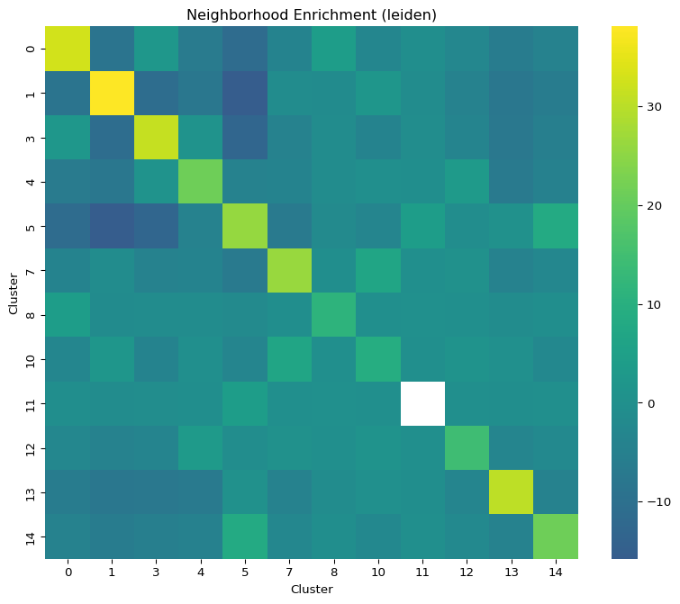
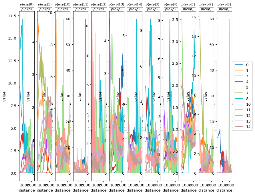
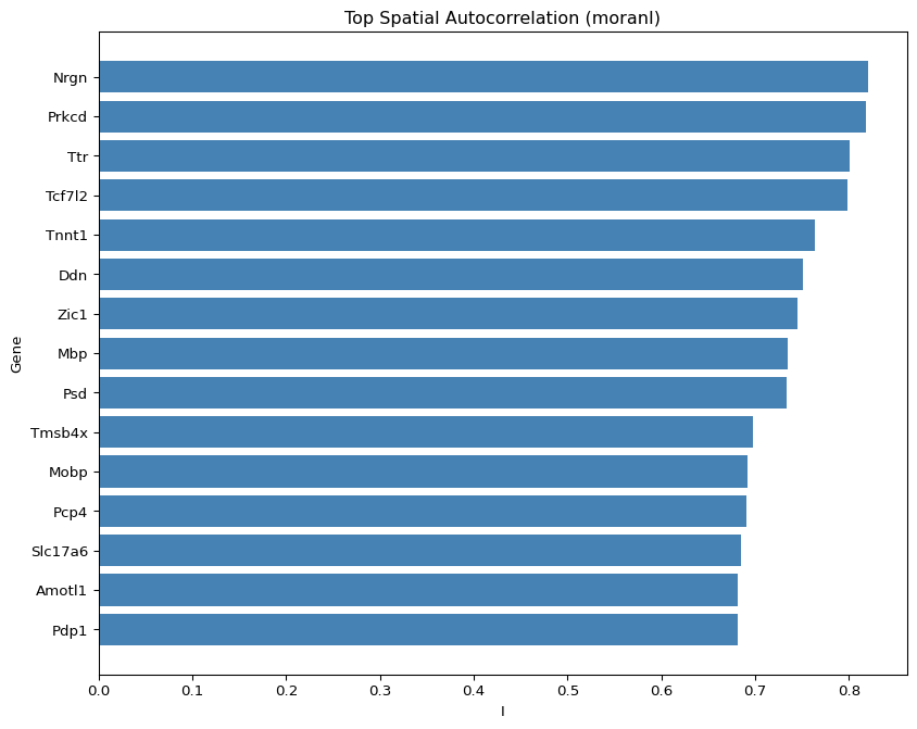
Nhood Enrichment, Spatial Graph Statistics and Co-Occurrence for who sits next to whom; Spatial Autocorrelation (Moran’s I, Geary’s C, or sepal on grids) and Spatial Hotspot for spatially variable genes and modules; Ripley L / F / G for point patterns.
- 08
Ligand–receptor and plots
Ligand-Receptor runs squidpy ligrec between cell types (its OmniPath intercell priors are installed via the Resource Center); Spatial Ligand-Receptor scores pairs per spot against the spatial graph. Spatial Visualization draws all of it, including H&E overlays, transcript density and the neighbour graph.
Every node, in pipeline order.
The app’s Node Library is modality-first: pick spatial transcriptomics and it shows these 50 nodes grouped into the 10 stages below. Shared nodes such as Quality Control or Merge Cell Meta appear in more than one view.
Stage 01
Load Data
11 nodes
Stage 02
QC & Preprocessing
7 nodes
Stage 03
Clustering & Embedding
6 nodes
Stage 04
Interactive Viewer
2 nodes
Stage 05
Neighborhood & Interaction
6 nodes
Stage 06
Tissue Structure
3 nodes
Stage 07
Spatial Statistics
3 nodes
Stage 08
Plots
2 nodes
Also available
Cell Type Annotation
3 nodes · collapsed by default in the app
Also available
Utilities & Export
7 nodes · collapsed by default in the app
Pre-wired pipelines — open, point at data, run.
Templates open from the Templates dialog with sensible defaults already set. Those marked below include a node whose database, model or manifest must be installed in the Resource Center first — every other node runs, and the gated one stops until it is installed. A run never downloads.
Spatial Neighborhood Analysis
4 nodesNeighborhood graph and enrichment on Visium mouse brain sample
Load H5AD → Spatial Neighbors → Nhood Enrichment → Spatial Visualization
Spatial Autocorrelation Scan
4 nodesLoad H5AD → Spatial Neighbors → Spatial Autocorrelation → Spatial Visualization
Spatial Full Analysis
19 nodesLoad H5AD → Highly Variable Genes → PCA → Neighbors → UMAP → Clustering → Spatial Neighbors → Nhood Enrichment → Co-Occurrence → Spatial Autocorrelation → Ripley → Ligand-Receptor → Spatial Visualization
Needs Resource Center install · Ligand-ReceptorMERFISH / MERSCOPE Spatial Analysis
9 nodesLoad CSV / TSV → Add Coordinates → Merge Cell Meta → Normalize → Log1p → Spatial Neighbors → Spatial Autocorrelation → Spatial Visualization
Sample data the templates point at
Paths are relative to the app’s sampledata/ folder.
sampledata/spatial/visium_mouse_brain.h5adVisium mouse brain section with obsm["spatial"] already populated.Used by: Spatial Neighborhood Analysis · Spatial Autocorrelation Scan · Spatial Full Analysis
What sets it apart
Native loaders, not hand-stitched coordinates
Visium (with H&E and true scalefactors), Visium HD (bin size as an explicit choice), Xenium, MERSCOPE and CosMx each have a loader that knows the vendor layout, so coordinates, images and control probes land where downstream nodes expect them.
Structure, not just statistics
BANKSY spatial domains and Schürch-style cellular neighborhoods sit next to squidpy’s neighborhood, co-occurrence, autocorrelation and Ripley tests — and NNLS deconvolution for spot data — on the same canvas.
Select regions by hand, keep them as data
Draw with lasso, box or polygon in the viewer, label the regions with Spatial Grouping, and the result is an ordinary obs column that Subset Data, DEG Analysis and every plot can use. The polygon geometry is saved with the workflow.
Local by design
Large runs stay on your machine; large result tables are streamed to the viewer rather than pushed into the node card. The optional AI Copilot sees node names, parameters and small summaries only.
Figures from this pipeline
3 captures
End matter
Start with Spatial today.
Free during the beta with an admin-issued Beta Access ticket. Windows 10/11, 64-bit. Runs locally; sign in at each launch.